Monday, December 30, 2013
R: how to debug the errors
options(error=recover): it will tell R to launch debug section and you can choose which one to debug
options(show.error.locations=TRUE): let R show the source line number
Something else:
use traceback() to locate where the last error message is and then use browser() to run the function again to check what is wrong.
Tuesday, December 24, 2013
A note about what is the output in predict.lm(lm_model, test_data, type=”terms”):
## first explain what is type="terms":  If type="terms" is selected, a matrix of predictions
## on the additive scale is produced, each column giving the deviations from the overall mean
## (of the original data's response, on the additive scale), which is given by the attribute "constant".

set.seed(9999)
x1=rnorm(10)
x2=rnorm(10)
y=rnorm(10)
lmm=lm(y~x1+x2)
predict(lmm, data=cbind(x1,x2,y), type="terms")

lmm$coefficient[1]+lmm$coefficient[2]*x1+mean(lmm$coefficient[3]*x2)-mean(y)-predlm[,1]
lmm$coefficient[1]+lmm$coefficient[3]*x2+mean(lmm$coefficient[2]*x1)-mean(y)-predlm[,2]
Monday, December 23, 2013
R: Calculate ROC and Plot ROC
library(ROCR)
library(Hmisc)

## calculate AUC from the package ROCR and compare with it from Hmisc

# method 1: from ROCR
data(ROCR.simple)
pred=prediction(ROCR.simple$prediction, ROCR.simple$labels)
perf=performance(pred, 'tpr', 'fpr')  #true positive and false negative
plot(perf, colorize=T)

perf2=performance(pred, 'auc')
auc=unlist(slot(perf2, 'y.values'))  # this is the AUC

# method 2: from Hmisc
rcorrstat=rcorr.cens(ROCR.simple$prediction, ROCR.simple$labels)
rcorrstat[1]  # 1st is AUC, 2nd is Accuracy Ratio(Gini Coefficient, or PowerStat, or Somer's D)
Monday, September 9, 2013
hadoop on cloudera quickstart vm test example 01 wordcount
Thanks to cloudera, we can test hadoop with its integrated tool kit (Cloudera QuickStart VM). it provides vmware, kvm and virtualbox edition to download. Everything is configured and you can test without any difficulty.
in this video, I show a example hot to do wordcount in hadoop. The youtube link is:
Steps not included in the video:
1: download vmware player or virtualbox and install;
2: download Cloudera QuickStart VM from cloudera(the link may change all the time, so you can google keyword "Cloudera QuickStart VM" to download).
The example of the wordcount test is:
1: install wget on centos server
sudo yum -y install wget
2: create test dir in /home/cloudera
mkdir /home/cloudera/test
cd /home/cloudera/test
3: create test txt file
echo "what can I do with hadoop on hadoop server or hive server" > test1.txt
4: put the txt file to hdfs
hdfs dfs -mkdir /user/cloudera/input
hdfs dfs -put /home/cloudera/test/test1.txt /user/cloudera/input/
5: go to /usr/lib/hadoop-mapreduce/
cd /usr/lib/hadoop-mapreduce/
6: run the job
hadoop jar hadoop-mapreduce-examples.jar wordcount /user/cloudera/input/test1.txt /user/cloudera/output
7: check what are there in the output
hdfs dfs -ls /user/cloudera/output/
8: reat the output file
hdfs dfs -cat /user/cloudera/output/part-r-00000
Thursday, August 15, 2013
proc sql: include redundant vars in select statement with group by
Wednesday, July 31, 2013
Fwd: Creating a Multidimensional Array for iris data
Thursday, July 25, 2013
The difference between BY and CLASS in PROC MEANS
CLASS and BY statements have similar effects but there are some subtle differences. In the documentation it says:
Comparison of the BY and CLASS Statements
Using the BY statement is similar to using the CLASS statement and the NWAY option in that PROC MEANS summarizes each BY group as an independent subset of the input data. Therefore, no overall summarization of the input data is available. However, unlike the CLASS statement, the BY statement requires that you previously sort BY variables.
When you use the NWAY option, PROC MEANS might encounter insufficient memory for the summarization of all the class variables. You can move some class variables to the BY statement. For maximum benefit, move class variables to the BY statement that are already sorted or that have the greatest number of unique values.
You can use the CLASS and BY statements together to analyze the data by the levels of class variables within BY groups.
Practically, this means that:
· The input dataset must be sorted by the BY variables. It doesn't have to be sorted by the CLASS variables.
· Without the NWAY option in the PROC MEANS statement, the CLASS statement will calculate summaries for each class variable separately as well as for each possible combination of class variables. The BY statement only provides summaries for the groups created by the combination of all BY variables.
· The BY summaries are reported in separate tables (pages) whereas the CLASS summaries appear in a single table.
· The MEANS procedure is more efficient at treating BY groups than CLASS groups.
options obs=10000;
libname temp "/data02/temp/temp_hsong/to_delete";
proc contents data=temp.high_vis_kws;
run;
proc sort data=temp.high_vis_kws out=high_vis_kws;
by nrank day_of_week;
run;
proc summary data=high_vis_kws;
by nrank day_of_week;
var clicks visits;
output out=classby1 sum=;
run;
proc summary data=high_vis_kws;
class nrank day_of_week;
var clicks visits;
output out=classby2 sum=;
run;
title "using by";
proc print data=classby1 width=min;
run;
title "using class";
proc print data=classby2 width=min;
run;
Tuesday, April 30, 2013
Distribution of The Difference of Two Uniform Distribution Variable
u1=runif(1000000,0,1)
u2=runif(1000000,0,1)

# Z is the difference of the two uniform distributed variable
z=u1-u2
plot(density(z), main="Density Plot of the Difference of Two Uniform Variable", col=3)

# X is the summation of the two uniform distributed variable
x=u1+u2
plot(density(x), main="Density Plot of the Summation of Two Uniform Variable", col=3)
Thursday, April 11, 2013
Read SAS data into R (SAS is required)
### To read SAS data into R(SAS is necessary) ##1: first use SAS to export data to csv or dlm, then use R
libname test "/data/temp/hsong/test";
proc export data=test.hsb12 outfile="/data/temp/hsong/test/sasxport" dbms=dlm replace;
delimiter=",";
run;
# Then read in the exported data with R read.table("/data/temp/hsong/test/sasxport", header=T)
##2: to read in with the package {Hmisc}
library(Hmisc)
hsb12=sas.get(lib="/data/temp/hsong/test", mem="hsb12", as.is=T)
##3: read with library {foreign}, but I did not run it successfully
read.xport("path")
use scan to read in a piece of data for ad-hoc analysis
A convenient way is to use scan function in R to directly read in the data by pasting them. Like:
x=scan(what=(list(a1=0,a2=0)))
y=data.frame(x)
Tips to incread the data reading speed in R
#The purpose is to compare the processing time when using different options to read in data with read.table
# test to read /data02/temp/temp_hsong/test/hsb12.sas7bdat
#1: without any options
system.time(read.table("/data02/temp/temp_hsong/test/sasxport.txt", header=T))
#2: By default R will convert character vars into factors wile reading
#suppress R convert character variables into factors by stringsAsFactors=F
system.time(read.table("/data02/temp/temp_hsong/test/sasxport.txt", header=T, stringsAsFactors=F))
#3: if data has no comment sign, then tell R
system.time(read.table("/data02/temp/temp_hsong/test/sasxport.txt", header=T, comment.char=''))
#4: roughly tell R a number slightly greater than the number of records
system.time(read.table("/data02/temp/temp_hsong/test/sasxport.txt", header=T, nrows=8000))
#5: When reading data, it's better tell R the mode of each var by colClasses
system.time(read.table("/data02/temp/temp_hsong/test/sasxport.txt", header=T, sep=',', colClasses=c(rep("numeric",11))))
Monday, April 1, 2013
The possible reason getting irregular coefficient(like we think it is positive, but it shows negetive)
The possible reason is we put high correlated variables in the predictors: suppose we have both sell_price and product_price in the model, and we know product_price is highly correlated to sell_price. An example is shown below in example 1.
Another possible reason is we recode the missing data: if missing data is at the left, but we recode it to the right(like if x<0 we recode x=99999 which is a very big number).
Example 1:
# set up random number seed set.seed(1000)
# generate 100 x with x ~ N(5,1) x=rnorm(100,5,1)

# Y=5*X y=5*x+rnorm(100,0,1)
# X1=100*X x1=x*100+rnorm(100,0,.2)

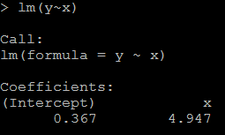
1)it is reasonable that the regression coefficient is 4.947(while the true value is 5). #relation between x and y lm(y~x)

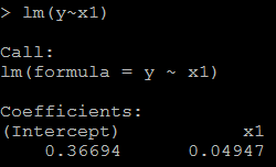
2) because x1=100*x, the coefficient for x1 should be 1/100 of above, as below: # relation between x1 and y lm(y~x1)

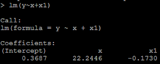
3) but if we put both x and x1 in the model, then we could not get the positive coefficient for both x and x1. This is because of multicollinearity. # put both x and x1 as the predictor lm(y~x+x1)

Example 2:
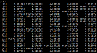
4) another condition is from we recode missing data. Suppose if x<=4 is missing, and we recode missing as 99999. # if x<=4, treat it as 99999 x3=ifelse(x>4,x,99999)

5) Then the regression coefficient is negative because of the 99999. # relation between x3 and y lm(y~x3)
The recode issue can be treated as a special case of non-linear relation.
Thursday, March 28, 2013
group obs almost evenly and calculate cumulative stats in SAS and R
The output is like:
In SAS, a loop is required to do this because of cumulative sum.
data test;
i=1;
p=.99;
output;
do i=2 to 98;
p=.8;
output;
end;
i=99;
p=.2;
output;
run;
proc print data=test;
run;
* if use proc rank, it cannot group data evenly because of ties;
proc rank data=test out=t group=10;
var p;
ranks rank;
run;
proc print data=t;
run;
* so need to mannuly do it;
%let dsid=%sysfunc(open(test)); *open the file;
%let nobs=%sysfunc(attrn(&dsid,nobs)); *count the obs in file; %let ngroup=10; %let overall_pct=.5; %put &nobs;
* data n_per_group only has one obs;
data n_per_group;
n_per_grp=int(&nobs/&ngroup.); * get quotient;
remainder=mod(&nobs,&ngroup.); * get remainder;
array ps {&ngroup} ps1-ps&ngroup;
keep ps1-ps&ngroup;
do i=1 to &ngroup;
if remainder>0 then do;
ps{i}=n_per_grp+1;
remainder=remainder-1;
end;
else ps{i}=n_per_grp;
end;
output;
run;
proc print data=n_per_group;
run;
* read in the only one obs, and keep it in PVM until the end by using if _n_=1 then do statement;
data out(drop=freq _count_ i p);
if _n_=1 then do;
set n_per_group;
index=1;
end;
retain freq _count_ 0 index ;
array ps(&ngroup) ps1-ps&ngroup;
set test end=last;
* a liitle tricky: keep on adding p together unitl the # of added obs = n_per_group as expected;
* if the # of added obs = n_per_group, calculate the stats we want, otherwise, keep on adding;
if _count_=ps(index) then do;
num_obs=ps(index);
avg_pred_p=sum_p/num_obs;
lift=avg_pred_p/&overall_pct;
output;
index+1;
_count_=0;
sum_p=0;
end;
sum_p+p;
_count_+1;
if last then do;
num_obs=ps(index);
avg_pred_p=sum_p/num_obs;
lift=avg_pred_p/&overall_pct;
output;
end;
run;
proc print data=out;
run;
## It is very easy to do this in R
## a simple way
rm(list=ls())
x=c(.9,rep(.8,97),.2)
ngrp=10
nobs=rep(length(x)%/%ngrp, ngrp)+c(rep(1,length(x)%%ngrp), rep(0,ngrp-length(x)%%ngrp))
levl=rep(1:ngrp, nobs)
df=data.frame(cbind(x,levl))
aggregate(x~levl, df, mean)


