Bayesian compution with R examples in SAS

学习了oloolo大拿的牛文，上面把 Bayesian compution with R 的例子全部改用sas写了一遍。一面学习oloolo的牛文，一面对照自己写一遍。中途写不出来的回去看看oloolo怎么写的，中间学了不少东西。呵呵，谢谢了。下面把自己尝试的code贴上。

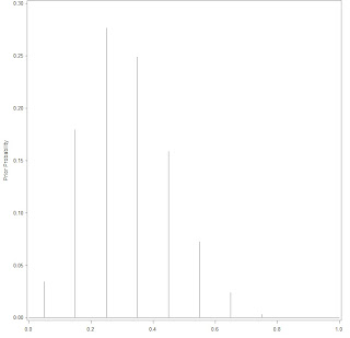
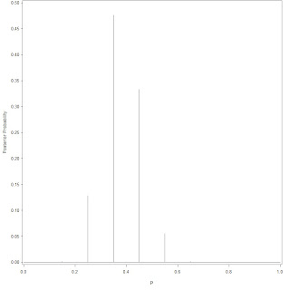
原来作者的R Code:

p = seq(0.05, 0.95, by = 0.1)
prior = c(1, 5.2, 8, 7.2, 4.6, 2.1, 0.7, 0.1, 0, 0)
prior = prior/sum(prior)
data = c(11, 16)
post = pdisc(p, prior, data)
round(cbind(p, prior, post),2)
library(lattice)
PRIOR=data.frame("prior",p,prior)
POST=data.frame("posterior",p,post)
names(PRIOR)=c("Type","P","Probability")
names(POST)=c("Type","P","Probability")
data=rbind(PRIOR,POST)
xyplot(Probability~P|Type,data=data,layout=c(1,2), type="h",lwd=3,col="black")

对应的SAS Code：

options fullstimer formchar='|----|+|---+=|-/\<>*'  formdlim='-'  error=3;
/***************************************************/
/*
模仿oloolo大牛的程序。把 Bayesian compution with R 中的例子用SAS写出来；
原文为oloolo所写；
用来练习，写不出来的，就看看oloolo怎么写的；
哈哈 :)
*/

/*
The following is to draw the graph for the discrete prior;
There are ten points that p may take, each with its weight respectively;
*/

data p;
    do p = .05 to .95 by .1;
        output;
    end;
run;


data prior;
input prior @@;
cards;
1  5.2  8  7.2  4.6  2.1  .7  .1  0  0
;
run;


data p;
    retain sum_prior 0;
    do until (eof1);
        set prior end = eof1;
        sum_prior + prior;
    end;
    do until (eof2);
        merge p prior end = eof2;
        prior = prior/sum_prior;
        output;
    end;
    drop sum_prior;
run;

goptions reset = all;
symbol interpol=Needle value=none line=1 color=black;
axis1 label = (angle = 90 'Prior Probability') order = (0 to 0.3 by .05) minor = none;
axis2 label = ('p') order = (0 to 1 by .2) minor = none;
proc gplot data = p;
    plot prior*p / vaxis=axis1 haxis=axis2;
run;
quit;

/*
Next is to calculate the posterior and then draw it;
*/

%let n0=16;
%let n1=11;

/*
Calculate the log-likelihood
*/
data p;  
 set p;
 if p > 0 and p < 1 then do;
     log_like = log(p)*&n1 + log(1-p)*&n0;
 end;
 else
     log_like = -999*(p=0)*(&n1 > 0) + (p=1)*(&n0 > 0) ;
run;

/*
Calculate the max(log-likelihood). Since exp(log_likelihood) is very colse to 0, if use it directly, almost all
calculated items is zero. So, use exp(log_likelihood - max), sacle the likelihood. It doesn't change the value
of likelihood since final likelihood = likelihood / sum(likelihood). If both numerator and denominator both
scaled by the same number, it doesn't change the fraction value.
*/
proc means data = p noprint;
    var log_like;
    output out = _max  max(log_like)=max;
run;

data p;
    set _max;
    sum_like = 0;
    do until (eof);
        set p end = eof nobs = ntotal;
        likelihood = exp(log_like - max);
        sum_like + likelihood;
    end;
    do until (eof1);
        set p end = eof1;
        likelihood = exp(log_like - max)/sum_like;
        posterior = likelihood * prior;
        output;
    end;
run;

data p;
    sum_post = 0;
    do until (eof);
        set p end = eof;
        sum_post + posterior;
    end;
    do until (eof2);
        set p end =  eof2;
        posterior = posterior / sum_post;
        output;
    end;
run;

goptions reset = all;
symbol interpol=Needle value=none line=1 color=black;
axis1 label = (angle = 90 'Posterior Probability') order = (0 to 0.5 by .05) minor = none;
axis2 label = ('p') order = (0 to 1 by .2) minor = none;
proc gplot data = p;
plot posterior*p / vaxis=axis1 haxis=axis2;
run;
quit;