Study Notes3 Predictive Modeling with Logistic Regression: group redundant variables

/* Redundant variables may degrade the analysis by: destabilize the estimation, overfitting, confounding*/

/* interpretation, and more computing time                                                              */

/* one solution for redundant variable is grouping the related variables                                */

/* proc varclus will find groups of variables that are as correlated as possible within groups and as   */

/* uncorrelated as possible with variables in other groups. Priciple component is done on the variables */

/* in each cluster by checking the Second Eigen Value. If it is greater than a given value, the cluster */

/* will be split into two child cluster. It's repeated until the SEV is less than the threshold         */

/* After the original variables are splited into different clusters, those clusters can be used to      */

/* replace the original variables as the predictors in the regression model, or a representative var    */

/* having high corelation with its own cluster and low correlation with the other clusters can be       */

/* selected from each cluster. The representative variable is picked by the 1-R^2 ratio                 */

/* 1-R^2 ratio = (1-R^2 of own cluster)/(1-R^2 of next cluster)                                         */

%let ex_inputs= MONTHS_SINCE_ORIGIN DONOR_AGE IN_HOUSE INCOME_GROUP PUBLISHED_PHONE

MOR_HIT_RATE WEALTH_RATING MEDIAN_HOME_VALUE MEDIAN_HOUSEHOLD_INCOME PCT_OWNER_OCCUPIED

PER_CAPITA_INCOME PCT_MALE_MILITARY PCT_MALE_VETERANS PCT_VIETNAM_VETERANS

PCT_WWII_VETERANS PEP_STAR RECENT_STAR_STATUS FREQUENCY_STATUS_97NK RECENT_RESPONSE_PROP

RECENT_AVG_GIFT_AMT RECENT_CARD_RESPONSE_PROP RECENT_AVG_CARD_GIFT_AMT RECENT_RESPONSE_COUNT

RECENT_CARD_RESPONSE_COUNT LIFETIME_CARD_PROM LIFETIME_PROM LIFETIME_GIFT_AMOUNT

LIFETIME_GIFT_COUNT LIFETIME_AVG_GIFT_AMT LIFETIME_GIFT_RANGE LIFETIME_MAX_GIFT_AMT

LIFETIME_MIN_GIFT_AMT LAST_GIFT_AMT CARD_PROM_12 NUMBER_PROM_12 MONTHS_SINCE_LAST_GIFT

MONTHS_SINCE_FIRST_GIFT    ;

proc varclus data=pva1 short hi maxeigen=.7 plots=dendrogram;

      var &ex_inputs mi_donor_age mi_income_group mi_wealth_rating;

run;

/* There are 23 clusters totally(based on the second egien value <= .7)                               */

/* Cluster one there are 5 variables, so total variation is 5. Variation explained by this cluster is */

/* 4.277752, which is about 85.56% of total variation. */

/* Those 23 clusters can be used as predictors directly, or a representative variable can be picked   */

/* from each cluster based on the 1-R^2 ratio. e.g., months_since_first_gift will represent cluster 1 */

Study Notes2 Predictive Modeling with Logistic Regression: collapse levels of contingency table

/* In the contingency table if there are many levels for a variable, then at some levels */

/* of this variable there may be no events(or all events) happening. This is called quasi */

/* completion problem(all separation). If this happens, the MLE will not exist since the */

/* regression coefficient will be infinit if want to maximize the likelihood */

/* A good solution is to collapse(cluster) some levels for the given categorical variable */

/*Variable Cluster_code has many levels which cause 0 events at some levels of cluster_code*/

/*This is called Quasi-completion problem*/

proc means data=pva1 nway missing;

class cluster_code;

var target_b;

output out=level mean=prop;

run;

proc print data=level width=min;

run;

ods output clusterhistory=cluster;

/* method=ward will use Greenacre's method to collapse levels of contingency tables */

/* the levels are clusterd based on the redunction in the chisq test of association */

/* levels with similar marginal response rate will be merged */

/* levels with least chisq value decreased will be merged, this is from the */

/* Semipartial R-Square value of the proc cluster output */

proc cluster data=level method=ward outtree=fortree plots=(dendrogram(vertical height=rsq));

freq _freq_;

var prop;

id cluster_code;

run;

proc freq data=pva1;

tables cluster_code*target_b / chisq;

output out=chi(keep=_pchi_) chisq;

run;

/* _pchi_ = 112.009 */

/* # of levels final is the one that giving least log(p_value) */

data cutoff;

if _n_ = 1 then set chi;

set cluster;

chisquare=_pchi_*rsquared;

degfree=numberofclusters-1;

logpvalue=logsdf('CHISQ',chisquare,degfree);

run;

proc sgplot data=cutoff;

scatter y=logpvalue x=numberofclusters / markerattrs=(color=blue symbol=circlefilled);

xaxis label="Number of Clusters";

yaxis label="Log of p-value";

title "Plot of the Log of p-value by Number of Clusters";

run;

/* number of clusters = 5 having the minimum logpvalue */

proc sql;

select numberofclusters into :ncl

from cutoff

having logpvalue=min(logpvalue);

quit;

ods html close;

proc tree data=fortree nclusters=&ncl out=clus;

id cluster_code;

run;

ods html;

proc sort data=clus;

by clusname;

run;

data clus_fmt;

retain fmtname "clus_fmt";

set clus;

start=cluster_code;

end=cluster_code;

label=clusname;

run;

/* at last use proc format to format the variable levels into clusters */

/* The formated fmt_cluster_code can be used as a categorical variable */

proc format cntlin=clus_fmt;

select clus_fmt;

run;

data pva1;

set pva1;

fmt_cluster_code=put(cluster_code,clus_fmt.);

run;

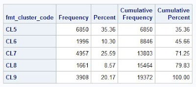
proc freq data=pva1;

table fmt_cluster_code / missing list;

run;

Study Notes1 Predictive Modeling with Logistic Regression: impute missing data with proc stdize for continuous variable

/*This is the study notes from SAS online training. It includes why use Logistic Regression, how to clean the data */

/*(impute missing value, cluster rare events levels, variable clustering, variable screening), how to build */

/*logistic regression and how to measure the performance of the model */

libname mydata "D:\SkyDrive\sas_temp";

proc datasets lib=mydata;

contents data=_all_;

run;

*** How to impute the missing data by proc stdize ***;

/*data preparation*/

data pva(drop=control_number);

set mydata.pva_raw_data;

run;

/*use proc means with nmiss to check how many obs are missing for each variable*/

proc means data=pva nmiss min max median;

var donor_age income_group wealth_rating;

run;

/*use array to set indicator for missing obs, if missing then indicatd as 1*/

data pva;

set pva;

array a_mi{*} mi_donor_age mi_income_group mi_wealth_rating;

array a_var{*} donor_age income_group wealth_rating;

do i=1 to dim(a_mi);

a_mi(i)=(a_var(i)=.);

end;

run;

/*group data into 3 groups by recent_response_prop from low to high: first 1/3 grp_resp is 0, next 1/3 of data is 1 */

/*the last 1/3 is 2. In the same way for grp_amt. So totally there are 9 groups of data considering grp_resp and grp_ant */

/*obs numbers in grp_resp level or grp_amt level are similar, but at grp_resp*grp_amt level is different */

proc rank data=pva out=pva groups=3;

var recent_response_prop recent_avg_gift_amt;

ranks grp_resp grp_amt;

run;

proc freq data=pva;

table grp_resp grp_amt / missing list;

table grp_resp*grp_amt / missing list;

run;

/*sort the data by grp_resp and grp_amt*/

proc sort data=pva;

by grp_resp grp_amt;

run;

/*impute the missing data in each group formed by grp_resp*grp_amt, by the median value of non-missing data in that group*/

/*after the imputation, the data will have imputed value as well as the missing value indicator */

proc stdize data=pva method=median reponly out=pva1;

by grp_resp grp_amt;

var donor_age income_group wealth_rating;

run;

/*check the imputed value in each group*/

proc means data=pva median;

class grp_resp grp_amt;

var donor_age income_group wealth_rating;

run;

/*there are some other ways to impute, like cluster imputation using proc fastclus */

/*or using EM, MCMC, Regression to impute in proc mi(see UCLA ATS) */

/*proc mi can also use logistic regression to impute the categorical variables */

/* http://www.ats.ucla.edu/stat/sas/seminars/missing_data/part1.htm */

/* http://www.ats.ucla.edu/stat/sas/seminars/missing_data/part2.htm */