Distribution of The Difference of Two Uniform Distribution Variable

Suppose U1~uniform(0,1), U2~uniform(0,1), and U1 is independent of U2, then what is the distribution of U1-U2?

The solution is in the picture attached. Then based on this, what is the distribution of U1+U2? The density should be of the same shape while it moves 1 unit to the right. The reason is: if U2 is uniform, then U3=1-U2 is uniform. so U1+U2 is the same as U1+U2=U1-U3+1. So it's density is the same as U1-U2 with i unit right transfer.

The answer can be verified in R. Density plot in R:

u1=runif(1000000,0,1)
u2=runif(1000000,0,1)
 
# Z is the difference of the two uniform distributed variable
z=u1-u2
plot(density(z), main="Density Plot of the Difference of Two Uniform Variable", col=3)
 
# X is the summation of the two uniform distributed variable
x=u1+u2
plot(density(x), main="Density Plot of the Summation of Two Uniform Variable", col=3)

Read SAS data into R (SAS is required)

Those 3 ways can read SAS data into R. I prefer the first method since it gives the most choice to control.

### To read SAS data into R(SAS is necessary)

##1: first use SAS to export data to csv or dlm, then use R

libname test "/data/temp/hsong/test";

proc export data=test.hsb12 outfile="/data/temp/hsong/test/sasxport" dbms=dlm replace;

        delimiter=",";

run; 

# Then read in the exported data with R

read.table("/data/temp/hsong/test/sasxport", header=T)

##2: to read in with the package {Hmisc}

library(Hmisc) 

hsb12=sas.get(lib="/data/temp/hsong/test", mem="hsb12", as.is=T)

##3: read with library {foreign}, but I did not run it successfully

read.xport("path")

use scan to read in a piece of data for ad-hoc analysis

Sometimes it is necessary to read in a piece of data for ad-hoc analysis. We can save the data to txt and then read in by read.table. In this way we need to find physical path of the data. It is not convenient for ad-hoc analysis especially when data is in server and R is in local machine.

A convenient way is to use scan function in R to directly read in the data by pasting them. Like:

x=scan(what=(list(a1=0,a2=0)))

y=data.frame(x)

Then do any analysis like plot and so on based on df y.

Tips to incread the data reading speed in R

Here are some tips to increase the data reading speed in R:

#The purpose is to compare the processing time when using different options to read in data with read.table

# test to read /data02/temp/temp_hsong/test/hsb12.sas7bdat

#1: without any options 

system.time(read.table("/data02/temp/temp_hsong/test/sasxport.txt", header=T))

#2: By default R will convert character vars into factors wile reading

#suppress R convert character variables into factors by stringsAsFactors=F

system.time(read.table("/data02/temp/temp_hsong/test/sasxport.txt", header=T, stringsAsFactors=F))

#3: if data has no comment sign, then tell R

system.time(read.table("/data02/temp/temp_hsong/test/sasxport.txt", header=T, comment.char=''))

#4: roughly tell R a number slightly greater than the number of records

system.time(read.table("/data02/temp/temp_hsong/test/sasxport.txt", header=T, nrows=8000))

#5: When reading data, it's better tell R the mode of each var by colClasses

system.time(read.table("/data02/temp/temp_hsong/test/sasxport.txt", header=T, sep=',', colClasses=c(rep("numeric",11))))

The processing time is:

The possible reason getting irregular coefficient(like we think it is positive, but it shows negetive)

Sometimes, we will get irregular coefficient: consider sell_amount vs sell_price, we should expect a negative coefficient because as the price increases, the selling amount should become less from common sense. But sometimes it may give a positive coefficient.

 

The possible reason is we put high correlated variables in the predictors: suppose we have both sell_price and product_price in the model, and we know product_price is highly correlated to sell_price. An example is shown below in example 1.

 

Another  possible reason is we recode the missing data: if missing data is at the left, but we recode it to the right(like if x<0 we recode x=99999 which is a very big number).

 

Example 1:

# set up random number seed

set.seed(1000)

# generate 100 x with x ~ N(5,1)

x=rnorm(100,5,1)

# Y=5*X

y=5*x+rnorm(100,0,1)

# X1=100*X

x1=x*100+rnorm(100,0,.2)

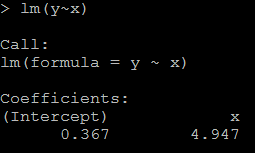
1)it is reasonable that the regression coefficient is 4.947(while the true value is 5). 

#relation between x and y

lm(y~x)

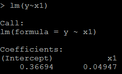
2) because x1=100*x, the coefficient for x1 should be 1/100 of above, as below:

# relation between x1 and y

lm(y~x1)

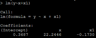
3) but if we put both x and x1 in the model, then we could not get the positive coefficient for both x and x1. This is because of multicollinearity. 

# put both x and x1 as the predictor

lm(y~x+x1)

Example 2:

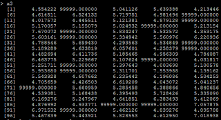
4) another condition is from we recode missing data. Suppose if x<=4 is missing, and we recode missing as 99999.

# if x<=4, treat it as 99999

x3=ifelse(x>4,x,99999)

5) Then the regression coefficient is negative because of the 99999.

# relation between x3 and y

lm(y~x3)

 

The recode issue can be treated as a special case of non-linear relation.